Plot the survival function — plot

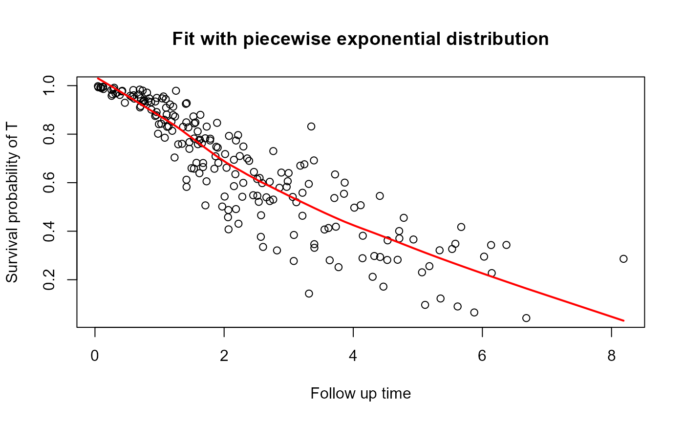
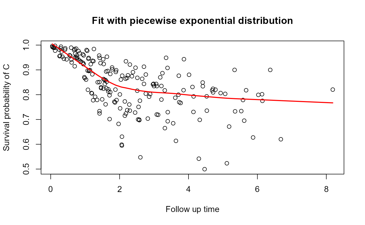
This graph helps to visualize the survival function.

Usage

plot_dc(object, scenario = c("t", "c", "both"))

Arguments

object: an object of the class "dcensoring".
scenario: which defines the scenario in the graph (t: failure times, c: dependent censoring times, or both).

Value

a survival function graph of the fitted model.

Details

In order to smooth the line presented in the graph, we used the 'lowess' function. So, it can result in a non-monotonous survival function.

Examples

# \donttest{
fit <- dependent.censoring(formula = time ~ x1 | x3, data=KidneyMimic, delta_t=KidneyMimic$delta_t,
                          delta_c=KidneyMimic$delta_c, ident=KidneyMimic$ident, dist = "mep")
plot_dc(fit, scenario = "both")


# }